Scan Mode
This topic provides descriptions of the parameters in the scan mode.
1. Data Acquisition Method
Description |
This parameter, together with the data acquisition buttons, determines how to generate data. |
||
|---|---|---|---|
Visibility |
Beginner, Expert |
||
Values |
|
||
Instructions |
When each option is selected, the functions of the data acquisition buttons are as follows:
|


2. Trigger Settings
Select the trigger sources and set relevant parameters.
| For the methods of triggering the laser profiler to acquire data in the scan mode, please refer to Methods for Triggering Data Acquisition. |
2.1. Data Acquisition Trigger Source
Description |
Select the source of the signals that trigger data acquisition. One round of data acquisition scans multiple lines of data, generates multiple profiles, and combines them into one image. |
|---|---|
Visibility |
Beginner, Expert |
Values |
|
Instruction |
|
2.1.1. Trigger Polarity
| This parameter is only visible when the Data Acquisition Trigger Source is set to Edge, Level, or Segmented Level. |
Description |
Sets the active direction or level state of the trigger signal. |
|---|---|
Visibility |
Expert |
Values |
|
Instruction |
|
2.1.2. Trigger Delay
Description |
Selects whether to set the trigger delay in time or line count. |
|---|---|
Visibility |
Expert |
Values |
|
Instruction |
After selecting the delay type, you need to set the corresponding Trigger Delay Time or Trigger Delay Line Count.
When Data Acquisition Trigger Source is set to Level you can also set the Trigger End Delay Time or Trigger End Delay Line Count corresponding to the Trigger End Delay.
|
2.1.3. Debounce Time
| This parameter is only visible when the Data Acquisition Trigger Source is set to Edge, Level, or Segmented Level. |
Parameter Description |
Sets the minimum valid duration of the input signal to filter out signal jitter and glitches. When the duration is shorter than this value, the signal is considered invalid and will not trigger acquisition. |
|---|---|
Visibility |
Expert |
Values |
|
Instruction |
Setting the debounce time too large may block valid signals. The parameter value should be set based on the pulse width of the valid external input signal. |
2.2. Line Scan Trigger Source
Description |
Select the source of the signals that trigger the scan of a single line. |
||
|---|---|---|---|
Visibility |
Beginner, Expert |
||
Values |
|
||
Instruction |
After selecting different options, different parameters are displayed in the Line Scan Trigger Source category for adjustment:
|
2.2.1. Trigger Rate
| This parameter is only visible when the Line Scan Trigger Source is set to Fixed Rate. |
Description |
When Line Scan Trigger Source is set to Fixed rate, set the fixed rate at which the laser profiler is triggered to scan. |
|---|---|
Visibility |
Beginner, Expert |
Values |
|
Instruction |
|
2.2.2. Trigger Delay Time
Parameter Description |
Sets the delay time between receiving a line scan trigger signal and emitting laser light. |
|---|---|
Visibility |
Expert |
Values |
|
Instruction |
|
Adjust Trigger Delay
In the following situation, you need to adjust Trigger Delay:
-
Multiple laser profilers are used to scan the same target object.
-
The line scans of all laser profilers are triggered by a single encoder.
-
The FOVs of the laser profilers overlap. The laser profilers will interfere with each other if they emit laser light at the same time.
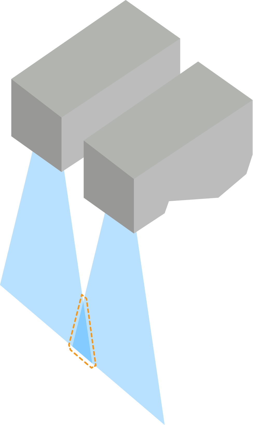
With an appropriate value of Trigger Delay, laser profilers emit laser light at different times and acquire data without interference.
|
Adjusting the value of Trigger Delay will have the following impacts:
|
Follow the steps below to adjust Trigger Delay:
-
Adjust the parameters of each laser profiler according to Preview Mode, Profile Mode, and Scan Mode, and ensure that the data acquired with each laser profiler meet the requirements.
-
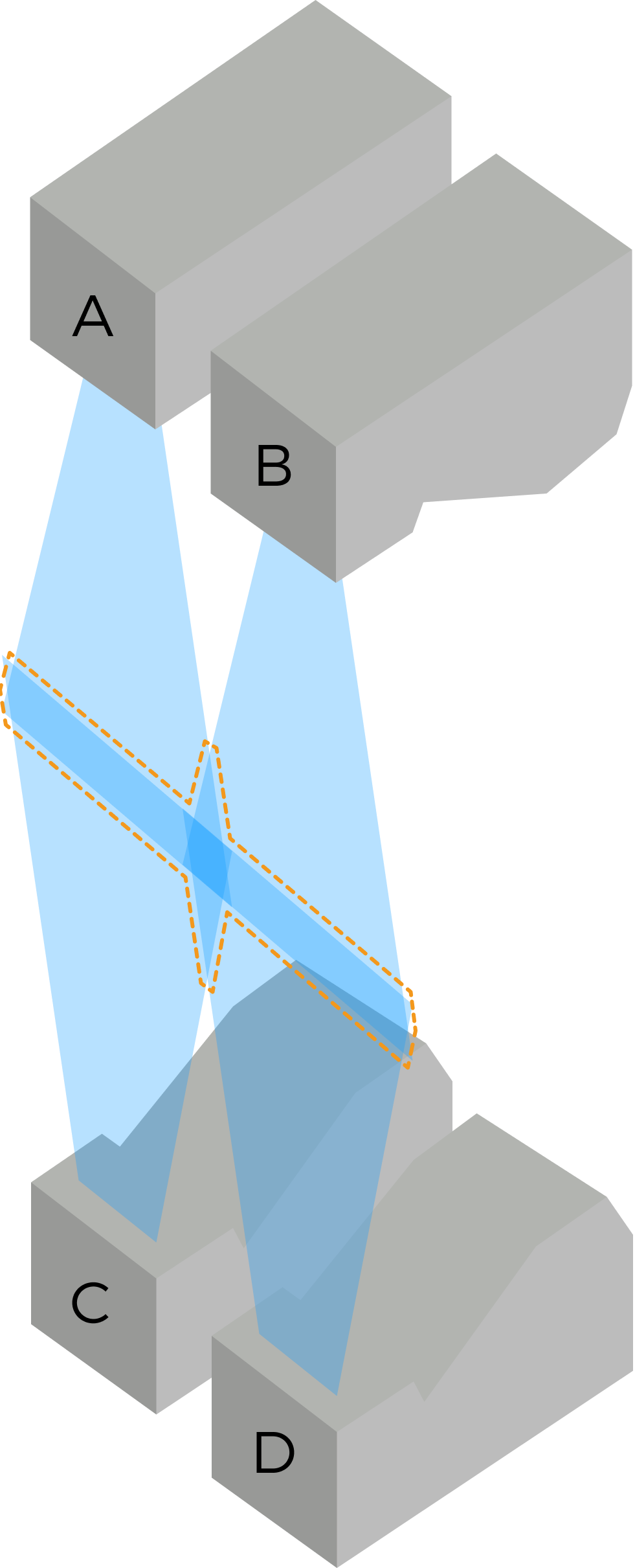
If more than two laser profilers are used, check the overlap of FOVs:
Overlap of FOVs
FOVs of all laser profilers overlap
FOVs of some laser profilers do not overlap (A and C in the image below)
Example of spatial relationship
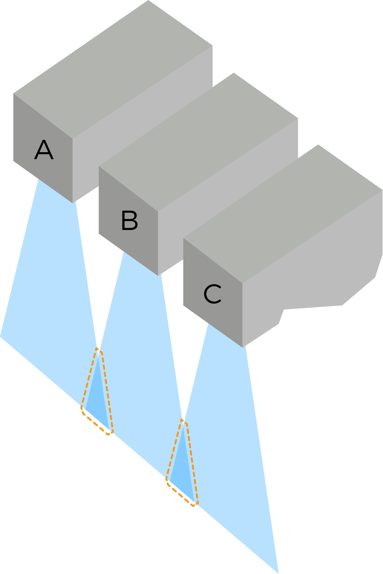
The purpose of adjusting Trigger Delay is to avoid interference in overlapping FOVs. Since laser profilers A and C in the image to the right of the table do not overlap, they can emit laser light simultaneously. You only need to adjust Trigger Delay for laser profiler B, making it emit laser light after laser profilers A and C.
-
Follow these steps to set Trigger Delay for laser profilers, referring to the spatial relationship examples and parameter settings in the table below:
-
Determine which laser profiler should emit laser light first, and keep the default Trigger Delay value of 0 for it.
-
Determine which laser profiler should emit laser light second, and set the value of Trigger Delay according to the following formula:
Trigger Delay = 10 μs + Exposure Time of the laser profiler first to emit laser light, window=_blank (Timed Exposure Mode), Exposure Time, window=_blank+Exposure Time2 (Dual-frame HDR Exposure Mode) or Total Exposure Time (Single-frame HDR Exposure Mode) in the HDR Exposure Settings.
The laser profiler starts exposure 10 μs after emitting laser light to ensure stable brightness of the laser lines in the raw image. -
Determine which laser profiler should emit laser light third, and set the value of Trigger Delay according to the following formula:
Trigger Delay = Trigger Delay of the laser profiler second to emit laser light + 10 μs + Exposure Time of the laser profiler second to emit laser light, window=_blank (Timed Exposure Mode), Exposure Time, window=_blank+Exposure Time2 (Dual-frame HDR Exposure Mode) or Total exposure time (Single-frame HDR Exposure Mode) in HDR Exposure Settings.
-
Set the value of Trigger Delay for all laser profilers following this logic.
Example of spatial relationship
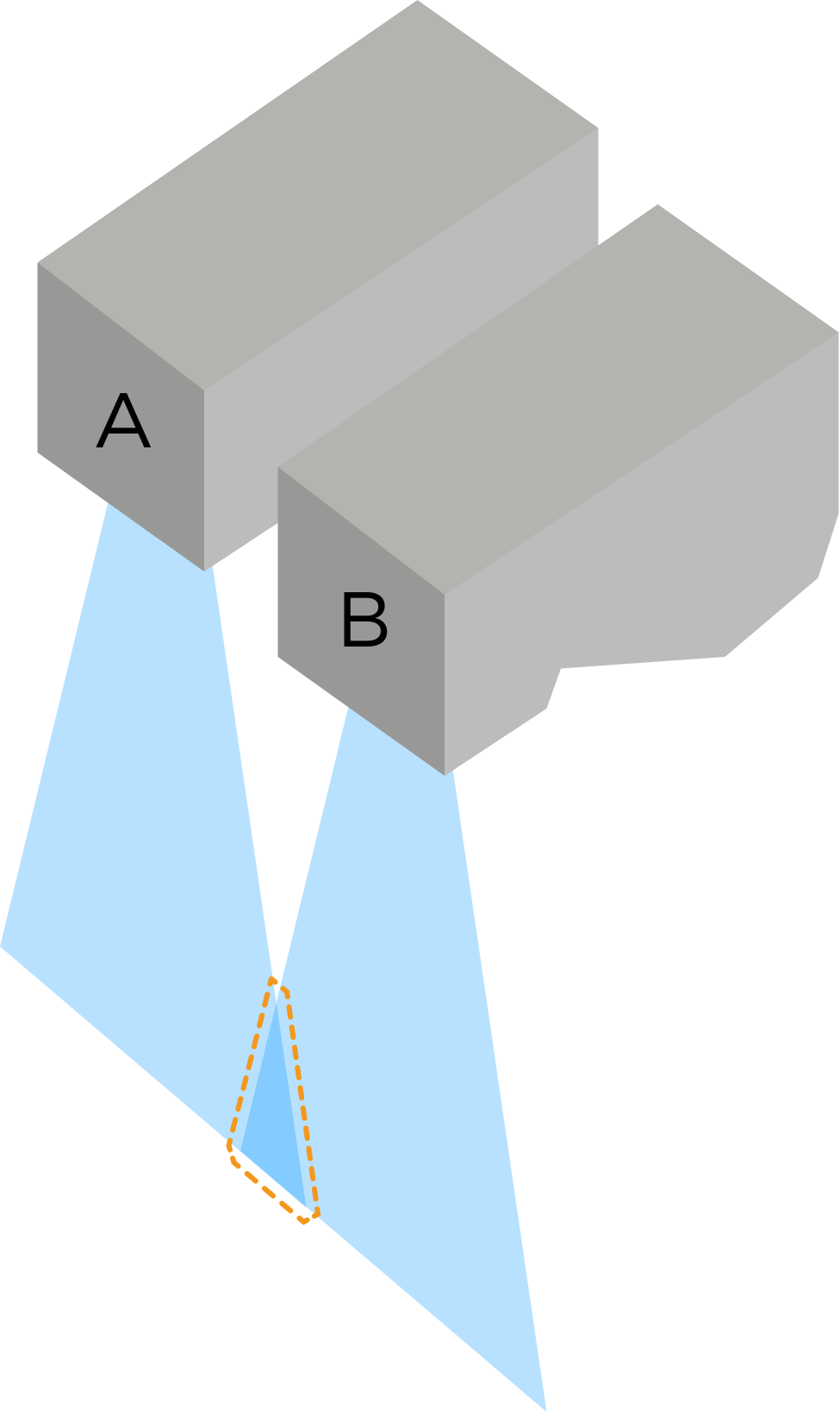
Parameter settings
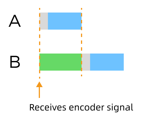
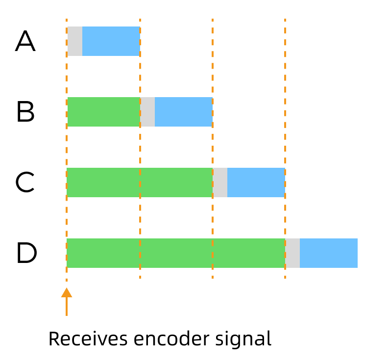
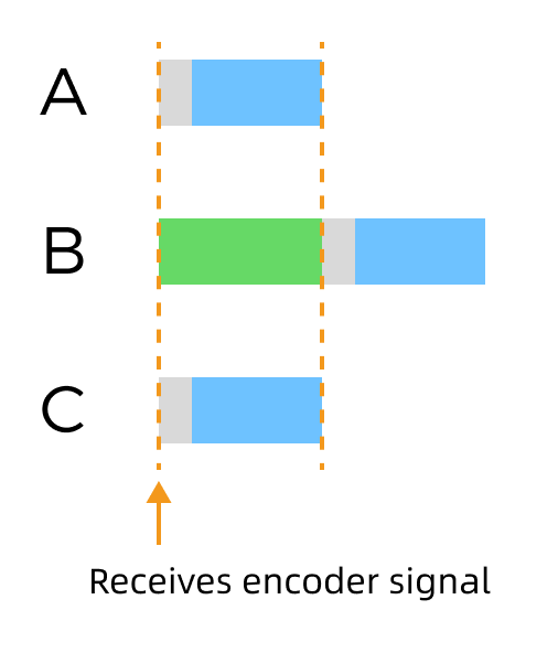
 : Exposure delay time:(10 μs)
 : Exposure Time/Total exposure time
 : Trigger Delay
-
2.2.3. Debounce Time
| This parameter is only visible when Line Scan Trigger Source is set to Encoder, Encoder A, or Encoder B. |
Parameter Description |
Sets the minimum valid duration of the input signal to filter out signal jitter and glitches. When the duration is shorter than this value, the signal is considered invalid and will not trigger acquisition. |
|---|---|
Visibility |
Expert |
Values |
|
Instruction |
Setting the debounce time too large may block valid signals. The parameter value should be set based on the pulse width of the valid external input signal. |
2.2.4. Encoder Settings
Parameters in this category need to be adjusted when Line Scan Trigger Source is set to Encoder or Encoder A/Encoder B.
Click Edit to open the Encoder Settings tool. You can check the encoder value and motion direction, and calculate the encoder resolution.
If you need the Y-axis resolution of the scan data to be equal to the X-axis resolution, you can also use this tool to get the recommended value of Trigger Interval.
① Trigger Direction
Description |
Select the encoder motion direction that triggers scanning. |
||||||||||
|---|---|---|---|---|---|---|---|---|---|---|---|
Visibility |
Beginner, Expert |
||||||||||
Values |
|
||||||||||
Instruction |
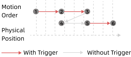
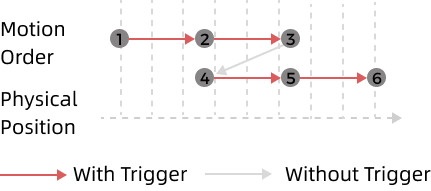
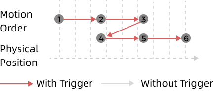
Adjust this parameter based on the encoder motion direction and the motion direction of the target object relative to the laser profiler.
|
② Trigger Signal Counting Mode
Description |
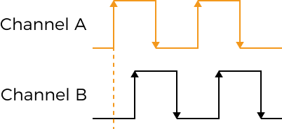
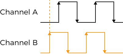
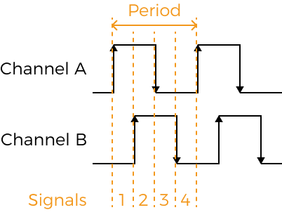
Set the number of quadrature signals to be counted in an encoder period. Counted signals are used to trigger scanning (These signals are trigger signals). Each encoder period contains 4 quadrature signals, as shown below.
|
||
|---|---|---|---|
Visibility |
Beginner, Expert |
||
Values |
|
||
Instruction |
This parameter and Trigger Interval together determine the rate at which scanning is triggered.
|
③ Trigger Interval
Description |
Set the number of trigger signals needed for scanning one line. |
||
|---|---|---|---|
Visibility |
Beginner, Expert |
||
Values |
|
||
Instruction |
This parameter and Trigger Signal Counting Mode together determine the rate at which scanning is triggered.
|
④ Trigger Interference Suppression
Parameter Description |
Enable this parameter to improve the trigger signal status and avoid false triggering caused by burst noise. |
|---|---|
Visibility |
Expert |
Values |
Enable the Trigger Interference Suppression switch:
|
Instruction |
In actual working conditions, such as unstable encoder signal sources or signal fluctuations caused by electromagnetic interference in the mechanism, false triggering may occur, affecting data acquisition. If you encounter such problems, it is recommended to enable this switch. |
2.3. Scan Line Count
Description |
This parameter sets the number of profiles in the acquired data. |
||
|---|---|---|---|
Visibility |
Beginner, Expert |
||
Values |
|
||
Instructions |
When the Data Acquisition Method parameter is set to Nonstop, this parameter sets the length of the returned data segments. |
2.4. Segmented Line Callback
Parameter Description |
Enable this parameter to output acquisition data in segments based on the configured line count. |
|---|---|
Visibility |
Expert |
Values |
Enable the Segmented Line Callback switch:
Callback Line Count: Sets how many lines of accumulated data are required to trigger one callback output. |
Instruction |
|
2.5. High Speed Mode
Parameter Description |
Enabling this parameter can improve the data acquisition speed, but the data quality may also decrease. |
|---|---|
Visibility |
Expert |
Values |
Enable High Speed Mode:
|
Instruction |
|
3. ROI
Parameter Description |
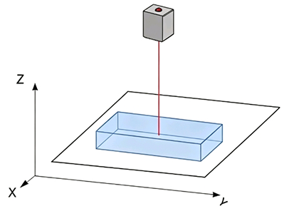
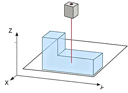
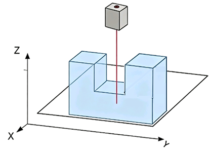
ROI defines the data processing range, reduces the amount of data to be processed, and enhances the max scan rate. Support setting a Fixed ROI on the X-Z plane or a Dynamic ROI that varies along the scan direction.
|
||||||||||||||
|---|---|---|---|---|---|---|---|---|---|---|---|---|---|---|---|
Visibility |
Beginner, Expert |
||||||||||||||
Values |
|
||||||||||||||
Instruction |
|
4. Interference Suppression
Parameters in this category are used to reduce interference factors and improve data quality and reliability.
4.1. Mask
Parameter Description |
Use masks to exclude unneeded data, such as noise and laser lines produced by interreflection. Masks are divided into Fixed Mask and Dynamic Mask.
|
||
|---|---|---|---|
Visibility |
Beginner, Expert |
||
Values |
Enable Mask toggle switch:
|
||
Instruction |
|
4.1.1. Edit Dynamic Mask
| Before using the Dynamic Mask tool, acquire depth data in the scan mode. |
After opening the Dynamic Mask tool window, follow these steps:
-
Enter the line range of each dynamic region in the Area List on the right, or drag the edge of the region in the image on the left for adjustment.
To add a dynamic region, click + Add; to delete it, click Delete to the right of the corresponding region. -
Click Next to open the dynamic mask editing window.
-
In the right Mask list, select the dynamic region to edit (such as Dynamic Region 1 Original Image ).
-
In the toolbar on the left, select the appropriate mask tool to add a mask to the image.
Please refer to Use Mask Tool for how to use the mask tool. -
If there are multiple dynamic regions, repeat steps 3 to 4 to edit the masks of other dynamic regions.
-
After configuration, click Apply to save the settings and exit the tool.
-
Acquire data again in the scan mode to check the effect of dynamic masks. If the result does not meet your requirements, please re-enter the tool and adjust it.
5. Dynamic Optimization
Parameter Description |
hen the surface properties of the target object vary significantly across different areas in the scan direction (e.g., black plastic and highly reflective metal), you can divide the scan direction into multiple areas and configure parameters for each area separately to meet different imaging requirements. |
|---|---|
Visibility |
Expert |
Values |
Default value: Disabled |
Instruction |
After enabling Dynamic Optimization, click the Edit button to the right of the Edit Dynamic Optimization area to open the Dynamic Optimization window and configure settings. For detailed instructions, please refer to Configure Dynamic Optimization below. h “Dynamic Optimization” is enabled, the following functions are unavailable in the preview mode:
|
5.1. Configure Dynamic Optimization Region
| Before using the dynamic optimization tool, acquire depth data in the scan mode. |
After opening the Dynamic Optimization window, follow these steps:
-
Enter a line range for the Dynamic Optimization area in the Region List on the right, or drag the edge of the area in the image on the left for adjustment.
To add a dynamic region, click + Add; to delete it, click Delete to the right of the corresponding region. -
Click the Next button to enter the Parameter Configuration interface.
-
In the Dynamic Optimization Region list on the left, select the region to be configured (such as Area0).
-
In the right Configure Parameters panel, you can select whether to display Dynamic Mask, to check the effect of masks in the current area.
Configure the following parameters according to the surface characteristics of the region:
-
If there are multiple regions, repeat steps 3 to 4 to configure the parameters in other regions.
Click the Region Parameter Configuration button next to the Dynamic Parameter Configuration  list on the left. You can view and modify the parameters of all regions in a centralized manner in the table.
-
After configuration, click Apply to save the settings and exit the tool.
-
Acquire data again in the scan mode to check the effect of dynamic optimization. If the result does not meet your requirements, please re-enter the tool and adjust it.
6. Resolution
Sets the X-axis resolution of the scan data and the Y-axis resolution of the point cloud.
6.1. X-axis Resolution
Description |
Sets the X-axis resolution of the scan data, which is the distance between two neighboring points along the direction of the laser line. |
|---|---|
Visibility |
Beginner, Expert |
Values |
|
Instruction |
|
6.2. Y-axis Resolution Mode
Parameter Description |
Select the mode for setting the Y-axis resolution. |
||
|---|---|---|---|
Visibility |
Beginner, Expert |
||
Values |
|
||
Instruction |
|
6.2.1. Y-axis Resolution
Parameter Description |
Sets the Y-axis resolution of the scan data, which is the distance between two neighboring points along the travel direction of the target object. |
|---|---|
Visibility |
Beginner, Expert |
Instruction |
When the Y-Axis Resolution Mode is set to Auto, this parameter is read-only and is calculated as follows:
|
6.2.2. Y-Axis Resampling Multiplier
Parameter Description |
Set the resampling multiplier of the scan data along the Y-axis. |
|---|---|
Visibility |
Expert |
Values |
|
Instruction |
Selecting 2× doubles the number of data rows through resampling; selecting 3× triples it, and so on. This parameter can be used to increase data density along the Y-axis. |
7. Correction
The parameters in this category are used to correct the height and direction deviations of the profiles.
|
Direction Correction is mutually exclusive with Tilt Correction and Height Correction. Once this option is enabled, other correction functions will be disabled. |
7.1. Tilt Correction
Parameter Description |
Correct the tilt of the profile, which is caused by the rotation of the laser profiler around the Y-axis. |
|---|---|
Visibility |
Beginner, Expert |
Values |
Enable Tilt Correction toggle switch:
Tilt Correction Angle:
|
Instruction |
For detailed instructions, refer to Tilt Correction. |
7.2. Height Correction
Parameter Description |
Correct the height error in the profile, which is caused by the rotation of the laser profiler around the X-axis. |
|---|---|
Visibility |
Beginner, Expert |
Values |
Enable Height Correction toggle switch:
Height Correction Ratio:
|
Instruction |
For detailed instructions, refer to Height Correction. |
7.3. Motion Direction Correction
Parameter Description |
This tool is used to correct the distortion in the point cloud caused by the inconsistency between the actual motion direction and the axis direction of the laser profiler. Motion direction is defined by the azimuth angle and elevation angle together. |
|---|---|
Visibility |
Beginner, Expert |
Values |
Enable the Motion Direction Correction:
Azimuth angle:
Elevation angle:
|
Instruction |
For detailed instructions, refer to Motion Direction Calibration. |
8. Point Cloud Optimization
The parameters in this category are used to optimize the generated point cloud. After adjusting the parameters, click Apply on the right to view the results.
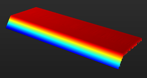
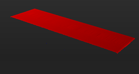
8.1. Normal filtering
Parameter Description |
Filters surface point clouds based on normal vectors to remove noise points caused by excessive surface undulation or steep edges. |
|---|---|
Visibility |
Beginner, Expert |
Values |
Enable Normal filtering switch:
Filtering Intensity:
|
Instruction |
Higher levels remove more noise but may result in greater detail loss. When selecting Customized, the following parameters need to be set. |
8.1.1. Custom Parameter Settings
| Parameters | Parameter Description | Value range | Default value |
|---|---|---|---|
Max Polar Angle |
Limits the upper limit of the angle between the normal vector and the Z-axis. Points whose normal vector forms an angle greater than this value are filtered out. |
0°~360° |
70° |
Min Polar Angle |
Limits the lower limit of the angle between the normal vector and the Z-axis. Points whose normal vector forms an angle less than this value are filtered out. |
0°~70° |
0° |
Min Z Angle |
Limits the lower limit of the angle between the normal vector projected onto the XY plane and the X-axis. Points whose normal vector forms an angle less than this value are filtered out. |
0°~360° |
0° |
Max Z Angle |
Limit the upper limit of the angle between the normal vector projected onto the XY plane and the X-axis. Points whose normal vector forms an angle greater than this value are filtered out. |
0°~360° |
360° |
Half Kernel Size |
Controls the neighborhood radius for normal estimation. A larger value produces smoother normals. |
0~30 |
2 |
Noise Removal Level |
As noise can be introduced by normal estimation, select the noise removal level according to the tolerance for noise removal. A higher level provides stronger noise removal. |
Close, Low, Medium, Height |
Low |
Smoothing Window Size |
Window size for mean smoothing. Apply mean smoothing to the surface data before filtering the normals to avoid abrupt normal changes due to noise. |
1~99 |
3 |
Point clouds before and after turning onNormal Filtering (all other conditions identical):
| Before | After |
|---|---|
|
|
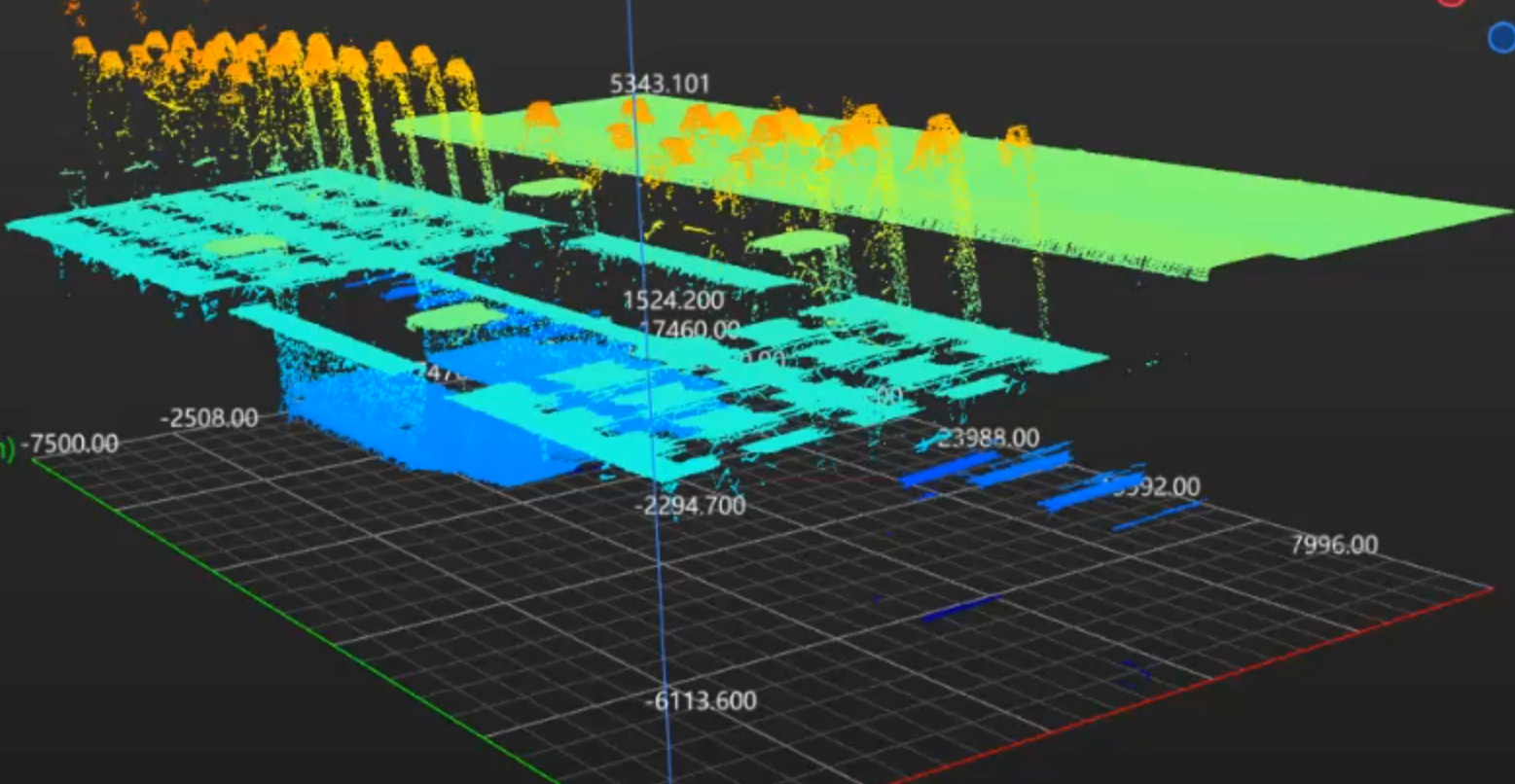
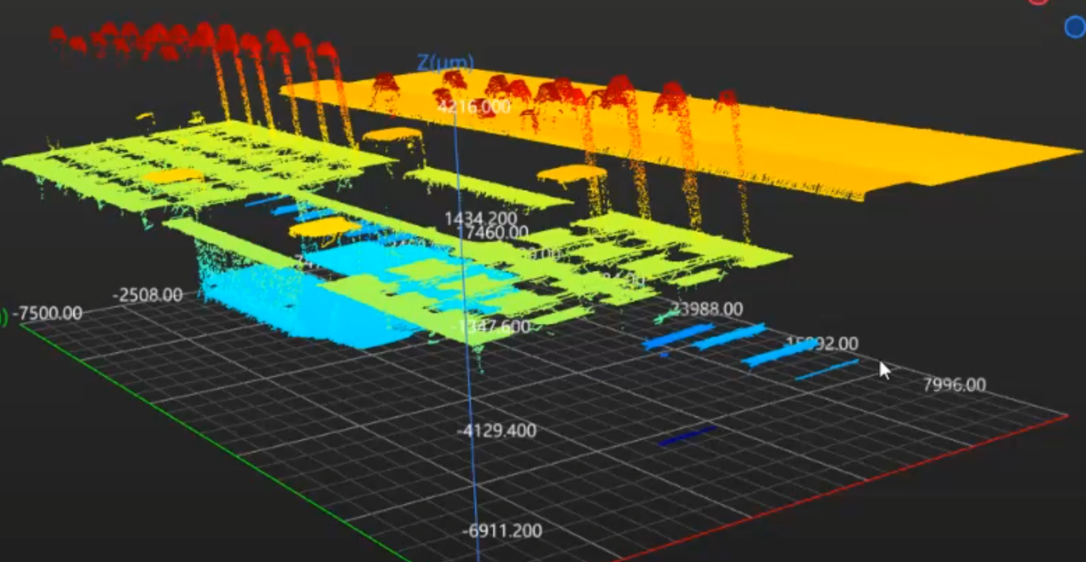
8.2. Connected Noise Removal
Parameter Description |
Remove small noise areas separated from the main point cloud. |
|---|---|
Visibility |
Beginner, Expert |
Values |
Enable Connected Noise Removal toggle switch:
Noise Removal Intensity:
|
Instruction |
Higher intensity removes more noise but may result in greater detail loss. When selecting Customized, the following parameters need to be set. |
8.2.1. Custom Parameter Settings
| Parameters | Parameter Description | Value range | Default value | ||
|---|---|---|---|---|---|
Depth Similarity Threshold |
Sets depth similarity threshold. If the depth difference between two neighboring points is less than or equal to this threshold, the points are considered similar and grouped into the same region. |
0~600 |
0.36 |
||
Neighborhood Type |
Determines which points around a point are considered its neighboring points. You can choose to identify the four immediate points above, below, left, and right of a point as its four neighbors, or identify the horizontal and vertical neighbors (as in 4-neighbor) and its four diagonal neighbors are its eight neighbors. |
|
8-neighbor |
||
Noise Detection Method |
Sets noise detection method. You can choose to judge whether it is a small noise region based on the number of points or size. |
|
Number of Points |
||
Max Noise Region Point Count |
Sets the maximum number of points for a region to be considered noise. If the number of points in a region does not exceed this value, the region is identified as noise and removed.
|
1~99999999 |
1000 |
||
Max size X/Y/Z |
Sets the maximum size for a region to be determined as noise in the X, Y, and Z directions, respectively.
|
X/Y:0~1000mm; Z:0~600mm |
2.0mm |
Point clouds before and after turning onConnected Noise Removal (all other conditions identical):
| Before | After |
|---|---|
|
|
8.3. Surface Noise Removal
Parameter Description |
Remove noise deviating from the main surface in the point cloud while preserving the effective surface structure as much as possible. |
|---|---|
Visibility |
Beginner, Expert |
Values |
Enable Noise Removal toggle switch:
|
Instruction |
After enabling, set the following parameters. |
8.3.1. Surface Type
Parameter Description |
Selects the expected surface type of the point cloud to be processed. This type will serve as the basis for surface noise detection. |
|---|---|
Visibility |
Beginner, Expert |
Values |
|
Instruction |
Please select the corresponding type according to the main surface morphology of the object to obtain more stable detection results. |
Plane Identification Strictness
When Surface Type is set to Plane, this parameter needs to be set.
Parameter Description |
Sets the strictness for removing noise based on plane features. A higher strictness requires the surface to match plane features more closely, so noise is removed only in regions that are closer to a plane, and fewer points are removed. |
|---|---|
Visibility |
Beginner, Expert |
Values |
|
Instruction |
|
8.3.2. Noise Removal Density
Parameter Description |
Sets the processing density for surface noise removal. A higher density provides more thorough noise removal but increases processing time. A lower density improves processing speed but may weaken the noise removal effect. |
|---|---|
Visibility |
Beginner, Expert |
Values |
|
Instruction |
|
8.3.3. Noise Removal Tolerance
Parameter Description |
Sets the tolerance for removing surface noise. A larger value makes noise removal less strict, so fewer points are removed. |
|---|---|
Visibility |
Beginner, Expert |
Values |
|
Instruction |
Increase this value appropriately when valid points are mistakenly deleted; decrease this value appropriately when there is too much residual noise. |
8.3.4. Surface Continuity Constraint
Parameter Description |
After this parameter is enabled, surface continuity is preserved as much as possible during noise removal to reduce surface breaks or holes. |
|---|---|
Visibility |
Expert |
Values |
Default value: Enabled |
Instruction |
Recommended for scenarios with high requirements for continuity; for more aggressive noise removal, compare the results with the disabled state. |
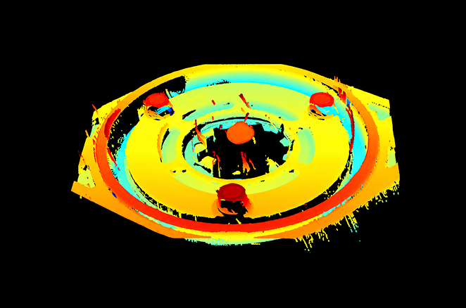
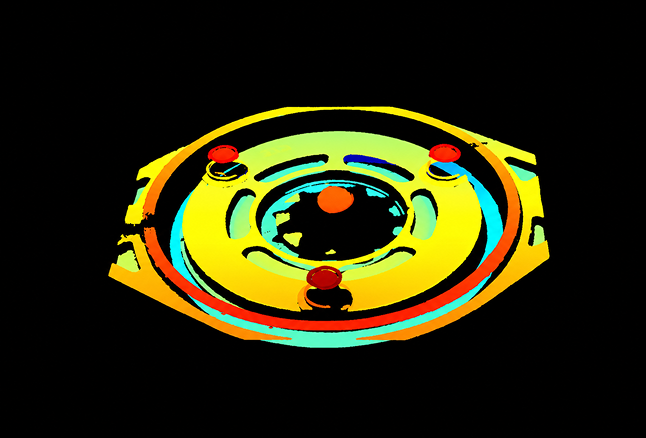
Point clouds before and after turning onSurface Noise Removal (all other conditions identical):
| Before | After |
|---|---|
|
|
8.4. Outlier Processing
Parameter Description |
Quickly removes outliers (flying points, isolated noise points, edge artifacts, etc.) from the point cloud and fills gaps. |
|---|---|
Visibility |
Beginner, Expert |
Values |
Enable the Outlier Processing switch:
Processing Intensity:
|
Instruction |
A higher level provides stronger noise removal and weaker gap filling. A lower level provides stronger gap filling and weaker noise removal. |
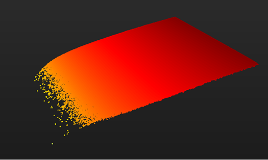
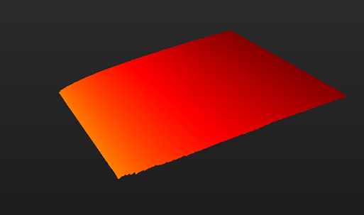
Point clouds before and after turning onOutlier Processing (all other conditions identical):
| Before | After |
|---|---|
|
|
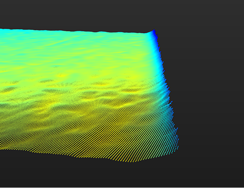
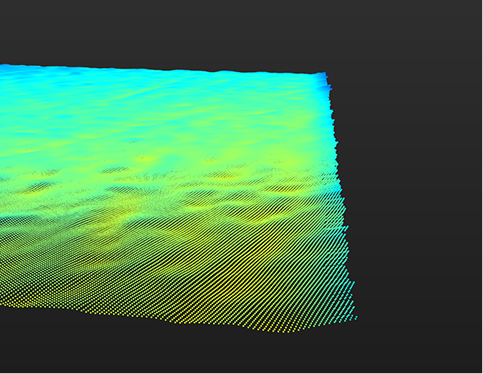
8.5. Edge Warping Suppression
The parameters in this group are used to suppress point cloud warping at object edges in scanned data.
The leading edge refers to the object edge at the start of scanning, and the trailing edge refers to the object edge at the end of scanning. Both sides can be configured independently.
8.5.1. Leading Edge Warping Suppression
Parameter Description |
Enable this parameter to detect and suppress warping in the leading-edge region at the end of scanning. |
|---|---|
Visibility |
Expert |
Values |
Enable the Leading Edge Warping Suppression switch:
|
Instruction |
After enabling, you need to set the Warping Line Count and Warping Direction below. |
8.5.2. Trailing Edge Warping Suppression
Parameter Description |
Enable this parameter to detect and suppress warping in the trailing-edge region at the end of scanning. |
|---|---|
Visibility |
Expert |
Values |
Enable Trailing Edge Warp Suppression switch:
|
Instruction |
After enabling, you need to set the Warping Line Count and Warping Direction below. |
Warp Height Threshold
This parameter is a shared threshold for Leading Edge Warping Suppression and Trailing Edge Warping Suppression.
Parameter Description |
Sets the height threshold for edge warping, which is defined as the height difference between the outermost point in the point cloud and the corresponding plane. Undulations exceeding this threshold are identified as warping. |
|---|---|
Visibility |
Expert |
Values |
|
Instruction |
The smaller the threshold, the more sensitive the judgment; the larger the threshold, the more relaxed the judgment. |
Warping Line Count
Leading Edge Warping Suppression and Trailing Edge Warping Suppression each have independent Warping Line Count parameters, which can be configured separately.
Parameter Description |
Sets the number of lines measured inward from the scan edge. Point cloud data within this range is used for warping detection and suppression. A larger value applies suppression to a wider edge region. |
|---|---|
Visibility |
Expert |
Values |
|
Instruction |
A larger value applies suppression to a wider edge region. |
Warping Direction
Leading Edge Warping Suppression and Trailing Edge Warping Suppression each have independent Warping Direction parameters, which can be configured separately.
Parameter Description |
Specifies the geometric direction of edge warping for more accurate suppression. |
|---|---|
Visibility |
Expert |
Values |
|
Instruction |
|
Point clouds before and after turning onEdge Warping Suppression (all other conditions identical):
| Before | After |
|---|---|
|
|
8.6. Uniform Smoothing
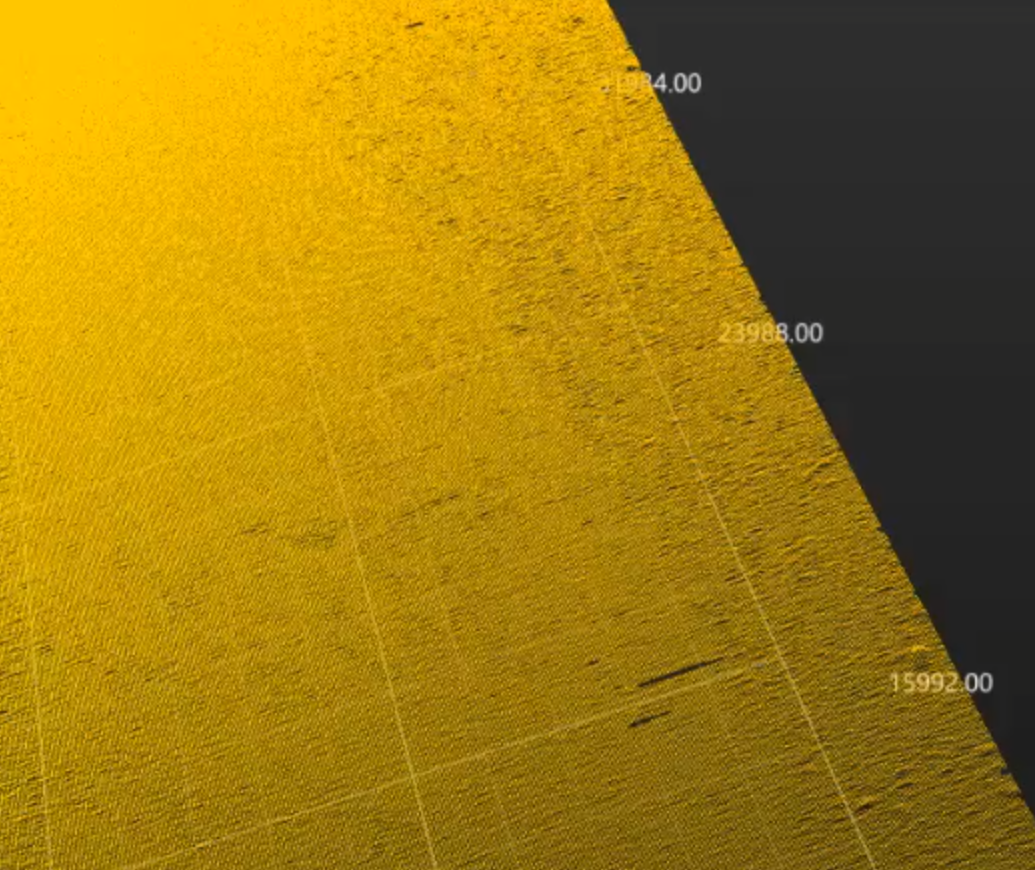
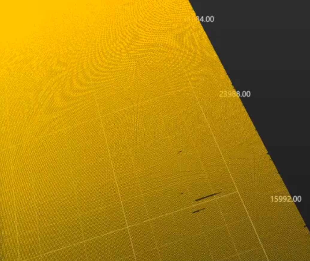
Parameter Description |
Perform uniform smoothing on the point cloud surface to reduce overall noise and depth fluctuations. |
|---|---|
Visibility |
Beginner, Expert |
Values |
Enable the Uniform Smoothing switch:
X-Axis Smoothing Intensity:
Y-Axis Smoothing Intensity:
|
Instruction |
A higher level produces stronger smoothing in X but weaker detail preservation.
|
Point clouds before and after turning onUniform Smoothing (all other conditions identical):
| Before | After |
|---|---|
|
|
8.7. Denoising Smoothing
Parameter Description |
Suppresses spike noise in the point cloud while largely preserving edge features. |
|---|---|
Visibility |
Beginner, Expert |
Values |
Enable the Denoising Smoothing switch:
X-Axis Smoothing Intensity:
Y-Axis Smoothing Intensity:
|
Instruction |
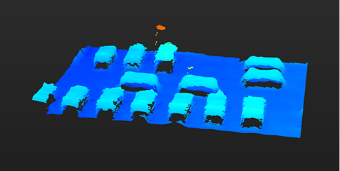
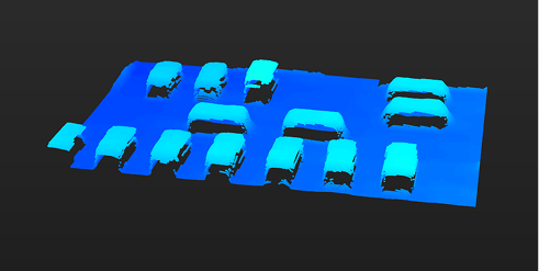
Higher levels provide stronger suppression of isolated noise points, but increase the risk of detail loss. When Custom is selected, X-Axis Window Size and Y-Axis Window Size must be set. Larger values suppress abnormal points over a wider range, but may weaken local details. |
Point clouds before and after turning on Denoising Smoothing (all other conditions identical):
| Before | After |
|---|---|
|
|
8.8. Gap Filling
Parameter Description |
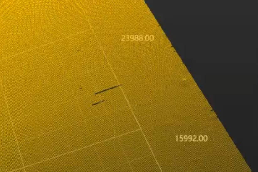
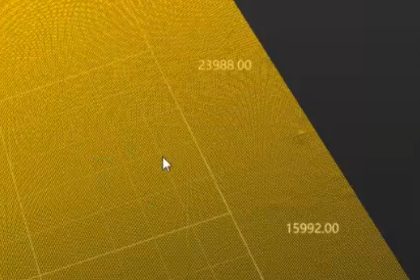
Fills missing regions in the point cloud caused by data loss, improving point cloud completeness. |
|---|---|
Visibility |
Beginner, Expert |
Values |
Enable Gap Filling:
X/Y-Axis Filling Window Size:
Filling Method:
|
Instruction |
|
Point clouds before and after turning on Gap Filling (all other conditions identical):
| Before | After |
|---|---|
|
|
8.9. Profile Alignment
The parameters in this category correct the X-axis and Z-axis vibrations in the profiles.
8.9.1. X-Axis Profile Alignment
Description |
This tool corrects the X-axis vibrations in the profiles. |
|---|---|
Visibility |
Expert |
Values |
Enable X-Axis Profile Alignment toggle switch:
|
Instruction |
Acquire data, and then click Edit to open the tool. For detailed instructions, refer to X-Axis Profile Alignment. |
Depth maps before and after turning on X-Axis Profile Alignment (all other conditions identical):
| Target object (demonstration) | Before | After |
|---|---|---|
|
|
|
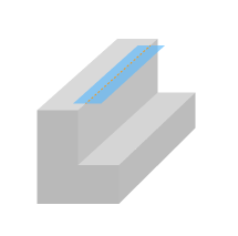
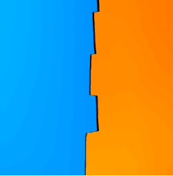
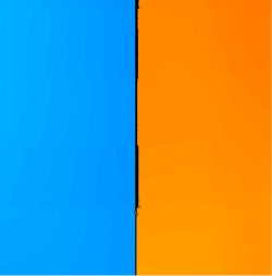
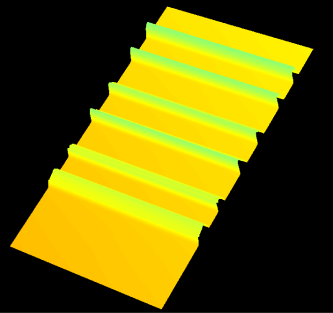
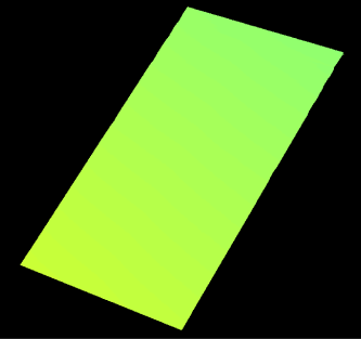
8.9.2. Z-Axis Profile Alignment
Description |
This tool corrects the Z-axis vibrations in the profiles. |
|---|---|
Visibility |
Expert |
Values |
Enable Z-Axis Profile Alignment toggle switch:
|
Instruction |
Acquire data, and then click Edit to open the tool. For detailed instructions, refer to Z-Axis Profile Alignment. |
Point clouds before and after turning on Z-Axis Profile Alignment (all other conditions identical):
| Target object (demonstration) | Before | After |
|---|---|---|
|
|
|
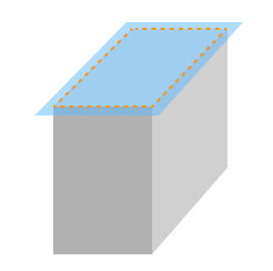
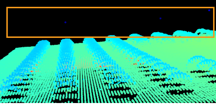
8.10. Enable Blind Spot Filtering
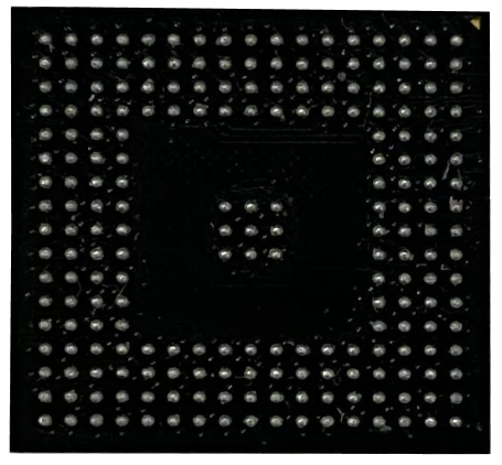
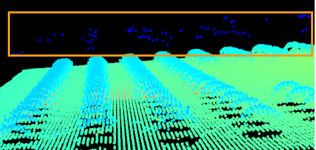
Blind spots are the areas on the target object surface where reflected laser lights are blocked.
However, if the surface of the target object has closely-spaced dents and bumps, such as PCBs, interreflection of the laser light might occur, thus producing false data near the blind spots. Interreflection can lead to incorrect data near blind spots. You can remove the false data by enabling the Blind Spot Filtering feature.
Description |
Identifies and removes false data caused by blind spots, thereby avoiding influence on further data processing. |
|---|---|
Visibility |
Expert, Guru |
Values |
Enable Blind Spot Filtering toggle switch:
Y-axis resolution: Displays the Y-axis resolution of the scan data. Filtering intensity: Displays the intensity of blind spot filtering.
|
Instruction |
Acquire data, and then click Edit to open the tool. For detailed instructions, refer to Blind Spot Filtering. |
Point clouds before and after turning on Blind Spot Filtering (all other conditions identical):
| Target object | Before | After |
|---|---|---|
|
|
|
8.11. Edge Preserving Smoothing
Parameter Description |
Reduces noise and depth fluctuations on the point cloud surface while preserving object edge details as much as possible. |
|---|---|
Visibility |
Beginner, Expert |
Values |
Enable the Edge Preserving Smoothing:
Smoothing Intensity:
|
Instruction |
A higher level produces stronger smoothing but weaker detail preservation on the object’s surface. |
Point clouds before and after enabling Edge Preserving Smoothing and Uniform Smoothing (all other conditions identical):
| Smoothing Disabled | Edge Preserving Smoothing | Uniform Smoothing |
|---|---|---|
|
|
|
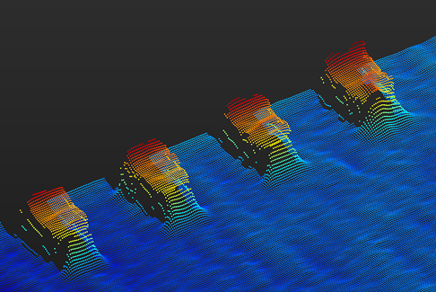
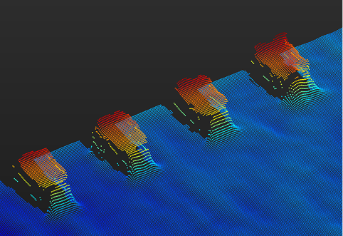
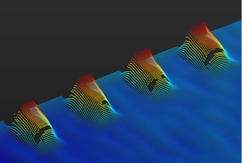
| Uniform smoothing applies the same intensity of smoothing to all areas, which weakens object edges and shape details; Edge preserving smoothing suppresses surface noise while preserving edge features. |
9. Data Output Settings
Parameters in this category are used to configure parameters related to output data, including sampling method, data type, and image enhancement parameters.
9.1. Sampling Method
Parameter Description |
Set the sampling method for data output. |
||
|---|---|---|---|
Visibility |
Beginner, Expert |
||
Values |
|
||
Instruction |
If you need to output the profile data with a fixed point spacing, select Uniform Spacing; if you need to keep the original sampling position, select Non-uniform Spacing.
|
9.2. Data Type
Parameter Description |
Set the type of output data. You can choose to output the intensity image or width image or not. |
|---|---|
Visibility |
Beginner, Expert |
Values |
|
Instruction |
Select the data type to be output according to the actual application requirements. |
9.3. Image Enhancement
Parameter Description |
Enhances image contrast and improves the display effect. Enable this parameter to apply the image enhancement effect to the image. |
|---|---|
Visibility |
Beginner, Expert |
Values |
Enable the Image Enhancement toggle switch:
|
Instruction |
You can enable this parameter when there is a requirement for the image display effect. Once enabled, you can adjust the enhancement parameters in Image Enhancement Settings. |
9.3.1. Image Enhancement Adjustment
Once Image enhancement is enabled, you can adjust the grayscale mapping curve and Gamma correction value through Image Enhancement Settings to optimize image contrast and overall brightness and darkness. These can be adjusted independently or combined for additive effect.
Please follow these steps:
-
Click Edit to the right of Image Enhancement to open the Image Enhancement Settings window.
-
Adjust the grayscale mapping curve: Drag knee points in the image or directly input the Input and Output values of the knee points below to adjust the mapping relationship between different grayscale intervals.
Click Reset to the right of Contrast to restore the default value of the curve. -
Set Gamma Correction Value: Adjust the Gamma Correction Value to adjust the overall brightness and darkness of the image. The larger the value, the darker the image. The smaller the value, the lighter the image.
-
After adjusting to the expected display, click Apply.
10. I/O Port Configuration
The parameters in this category are used to configure the input and output signals of the I/O ports of the laser profiler.
10.1. Configurable I/O
Bidirectional port that can be configured as input or output. Select the corresponding function based on the signal direction.
10.1.1. Mode
Parameter Description |
Sets the signal direction of the configurable I/O. |
|---|---|
Visibility |
Expert |
Values |
|
Instruction |
|
10.1.2. Function
Parameter Description |
Sets the function of the configurable I/O. The available options will change according to the Modesettings. |
|---|---|
Visibility |
Expert |
Values |
When Mode is Input:
When Mode is Output:
|
Instruction |
|
10.1.3. Polarity Inversion
Parameter Description |
Inverts the signal logic of the configurable I/O. In Input mode, it affects the trigger edge; in Output mode, it affects the output level. |
|---|---|
Visibility |
Expert |
Values |
Enable the Polarity Inversion switch:
|
Instruction |
When enabled, reverses the polarity of the output signal. In Output Mode, high level and low levels are swapped; in Input Mode, rising and falling edges are swapped. |
10.2. Output 1 and Output 2
Sets the behavior of output port, including trigger event and signal polarity.
10.2.1. Event
Parameter Description |
Selects the event type that triggers the output signal. |
|---|---|
Visibility |
Expert |
Values |
|
10.2.2. Polarity Inversion
Parameter Description |
When enabled, the level logic of the output signal is reversed, meaning high becomes low, and low becomes high. |
|---|---|
Visibility |
Expert |
Values |
Enable the Polarity Inversion switch:
|